Data Mining Non Stationarity And Entropy
This paper provides simple intuitive explanations for three interrelated concepts that have provocative, implications for investment management: data mining, non-stationarity, and information entropy.
By Bradford Cornell
Introduction
This paper provides simple intuitive explanations for three interrelated concepts that have provocative, implications for investment management: data mining, non-stationarity, and information entropy. The first two have been extensively analyzed in the literature and the point of this article is not to review that work, but to provide nontechnical explanations that highlight the investment implications. Information entropy has not been analyzed as widely but turns out to be closely related to the other two issues.
Data Mining
To illustrate how data mining issues arise in investment analysis, consider the example of the expansion of pi. Pi provides a noncontroversial illustration because extensive analysis has determined that there are no patterns, or to use the term from the investment literature no “anomalies,” in the sequence of digits. Therefore, any apparent anomaly must be the result of data mining.
As one example, it is alleged that as a youth famed physicist Richard Feynman used to like to reel off the first 767 digits of Pi, at which point there is a sequence of 9-9-9-9-9-9, and then say, “and so on.” For this reason, the sequence of six 9’s is known as the Feynman point. How anomalous is this pattern? Is it meaningful evidence of non-randomness? The answer depends critically on what is meant by “this pattern.”
If ex-ante the prediction was that there would be a sequence of six 9’s in the first 800 digits of the expansion of pi, the confirmation of the prediction would be significant evidence of non-randomness. The probability is less than 0.0001. But no one made that prediction ex-ante. The sequence was simply observed ex-post. With regard to ex-post observations, there is nothing unique about six 9s. The same conclusion would have been drawn for any other string of six identical digits. Similarly, what about a rising sequence like 1-2-3-4-5-6 or a declining sequence of the same type, these outcomes seem equally “anomalous.” The reader can no doubt think of other anomalies like the first day of the new millennium 1-1-2000. The point is that if the anomaly is not defined specifically ex-ante, the probability that some anomaly will be found becomes almost certain. In the case of the first 800 digits, the specific anomaly happened to be six 9’s.
Furthermore, there is nothing unique about the first 800 digits. For instance, if you pick the right place in the expansion, you can find the sequence 0-1-2-3-4-5-6-7-8-9. That sequence starts at digit 17,387,594,880. There is even free software on the internet that will find your birthdate in the expansion of pi.
What makes data mining such a problem in finance are two issues. First, there is no way to expand the data by doing new experiments. Even though there is only one expansion of pi, it is infinite so new sequences can always be found to test whether the discovery of a proposed pattern is spurious. Finance is not so lucky – there is only one fixed historical sample. Second, there are too many asset pricing models. As a result, once an anomaly is observed, there is a plethora of models, including behavioral alternatives, to choose from to explain the observation. And if an existing model cannot be found, it is always possible to invent a new one.
Recognition of these data mining problems is widespread. In his Presidential address to the American Finance Association, Campbell Harvey (2017) noted that the combination of the search for significant anomalies, the large number of researchers with the need to publish, and the existence of one data set makes the risk of data mining particularly serious. More specifically, he said, Given the competition for top journal space, there is an incentive to produce “significant” results. With the combination of unreported tests, lack of adjustment for multiple tests, and direct and indirect p-hacking, many of the results being published will fail to hold up in the future. In addition, there are basic issues with the interpretation of statistical significance. Going further, Harvey (2021) points out that over 400 factors (strategies that are supposed to beat the market) have been published in top academic journals.
Finally, it is worth noting that improvements in computer hardware and machine learning algorithms are a mixed blessing. Although machines can find patterns that humans will miss, they can also find spurious patterns that humans rightly overlooked.
To be sure there are things that can be done to combat data mining. Harvey (2021) suggests several such as: (1) Be aware of how many different specifications were tried, (2) Be cognizant of the incentives involved in the research project, (3) Make sure that the investment strategy suggested by the research has a solid economic foundation (4) Require higher levels of statistical significance when interpreting the results. If data mining were the sole issue, its impact could be ameliorated by following suggestions such as those offered by Harvey, but it is not the only problem. The second problem, non-stationarity, may even present a bigger obstacle.
Non-stationarity
From an investment standpoint the problem of data mining amounts to finding spurious “patterns” in asset prices. The problem of non-stationarity is finding patterns in asset prices that existed in the past but are no longer there.
Formally, a stationary stochastic process is one for which the joint probability distribution does not change when shifted in time. Consequently, parameters such as the mean and the variance also do not change over time. The formal definition is hard to grasp intuitively. A better approach is to think in terms of drawing colored balls from jugs.
Consider the following thought experiment. You are given a large jug which is known to contain an assortment of colored balls. You are allowed to make a series of draws from the jug, note the color of the ball, and then replace it. The jug is then shaken (randomized) and the experiment is repeated. The question is what can be learned from this process? The law of large numbers implies that with a sufficient number of draws, it is possible to estimate the relative fraction of balls of each color, which equals the probability of drawing that color on the next trial, with accuracy that converges to certainty.
The sequence of draws is an example of a stationary process. There is no change over time in process by which balls are drawn. Contrast this with a situation where nature chooses the jug from a sample of n jugs. After the jug is chosen, the experimenter draws a ball and notes the color. Each of the n jugs, in turn, contain differently colored balls in different proportions. Under such circumstances, it is possible to conceive of a two-step stationary process. If nature follows a stationary process for choosing the jugs, say picking a random number between 1 and n, then the two-step process of choosing a jug and a ball will be stationary. With sufficient repetitions, the experimenter can determine the relative frequency of each color ball in the aggregate sample of all n jugs, but not the number in each jug. For instance, with two jugs the experimenter could learn that half the balls are red and half are blue in the aggregate but cannot determine if this is because each jug contained half red and half blue balls, or one jug was all red and the other all blue, or any combination that summed to half red and half blue.
The situation becomes increasingly daunting as n grows and when it can no longer be assumed that nature follows a stationary process for choosing among the jugs. Furthermore, if the number of times the experiment can be repeated is limited, that further reduces what can be learned about the underlying processes generating the sequence of draws. Under such circumstances, it is no longer possible to estimate the probabilities regarding the colors of future balls.
The two cases correspond to Knight’s (1921) distinction between risk and uncertainty. Risk applies to the one jug example where the probability distribution of future draws can be determined. Uncertainty is a situation in which the world is sufficiently non-stationary that even the probability distribution cannot be reliably estimated. That corresponds to the situation in which n is large, the procedure nature uses for choosing the jugs is subject to random variation, and the number of times the experiment can be repeated is limited.
To draw an analogy with investing, the jugs can be interpreted as the “market environments,” including risk preferences, investment opportunities, investor sentiment, behavioral biases, and all other relevant data necessary to describe market conditions. The ball drawn can be interpreted as random vector of security returns conditional on the chosen market environment. The stochastic properties of the return vector including its mean and covariance matrix depend on the jug nature selects – the market environment.
If the world is described by the one jug example, then the probability distribution of the return vector can be determined. This is the effective assumption made by many asset pricing models. In the intermediate case where there is a two-step process that is stationary, investors would be able to determine the stochastic properties of the long-run vector of returns, but not the vector of returns conditional on the current state of the world. If the non-stationarity is too severe, then even the properties of the long-run vector of returns, or other state variables, cannot be learned with confidence. The critical questions are where the real world lies along this spectrum, how can we tell where it lies, and what implications does that have for investors?
Combining data mining and non-stationarity
The fact that both data mining and non-stationarity typically interact further complicates investment decision making. If a strategy based on historical data fails to deliver as expected it could be due to data mining (the historical pattern was a mirage), non-stationarity (the historical pattern disappeared), or any combination of the two. Furthermore, the interaction between the two is likely to vary across investment strategies and over time. The demise of the value effect provides an example.
Prior to 2007 the value effect was perhaps the most extensively documented asset pricing “anomaly.” For instance, Dimson, Marsh and Staunton (2020), in their comprehensive annual update on global market returns, noted that the value premium (the premium earned by low price to book stocks, relative to the market) has been positive in 16 of the 24 countries that have returns for more than a century and amounted to an annual excess return of 1.8%, on a global basis. The value premium was so widely accepted that it set off a debate regarding whether the premium was evidence of mispricing or an indication that asset pricing models needed to be adjusted to account for unappreciated risks. Most notably, Fama and French (1992) argued that the value premium reflected a risk premium whereas Lakonishok, Shleifer, and Vishny (1994) claimed it was evidence of behavioral based mispricing. But neither side disputed the evidence of the existence of the premium
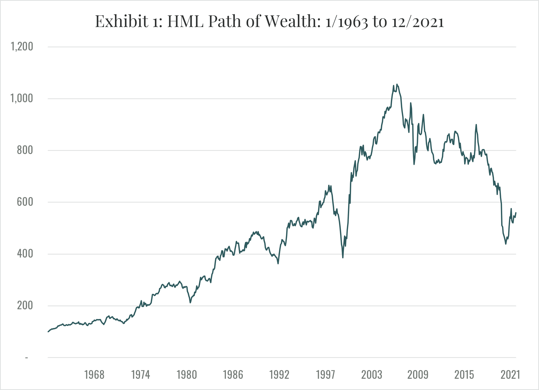
Then, beginning in 2007, the premium disappeared. The extent of value’s demise depends on how it is measured, but all measures produce the same general picture. One common metric is the return on the zero net investment HML portfolio (long high book to market, short low book to market) originally constructed by Fama and French (1992) and regularly updated by Prof. French on his website. Exhibit 1 plots the path of wealth (POW) derived from the HML portfolio returns from January 1963 through December 2021. Except for a dip during the dot.com bubble, the exhibit shows the inexorable rise in the POW resulting from a continuing value premium until about 2007. At that point, a volatile decline begins, and the POW drops to less than half of its 2007 maximum before recovering slightly.
Although the disappearance of the value effect is perhaps the most dramatic example of the demise of an investment strategy, it is hardly unique. In a recent paper, Asness (2020) reaches the same conclusion with respect to the size effect. In a similar vein, Banegas and Rosa (2022) challenge the reliability of momentum-based strategies. More generally and as noted earlier, Harvey (2021) reports that over 400 factors (strategies that are supposed to beat the market) have been published in top journals. How could that be possible in a competitive market? Hou, Xue and Zhang (2020) find that 65% of the 452 anomalies in their extensive data library, including 96% of the trading frictions category, cannot clear the single test hurdle for replication of an absolute t-value of 1.96. The point here, however, is not to offer a thorough review of the replication debate. It is simply to emphasize the potential impact of data mining and non-stationarity for the reliability of investment strategies based on observed historical patterns in returns.
Entropy
The statistical concept of entropy began with the work of Boltzmann in the 19th century. Boltzmann distinguished between the macrostate of a system, such as a mole of gas, and the microstates of the system. The macrostate is what is observable, such as the mass, pressure, volume, and temperature of the gas. The microstates consist of all the possible configurations of the molecules of the gas consistent with a given macrostate. For a mole of gas, the number of microstates is a mind-bogglingly huge number. If each molecule can be in X states (defined, for instance, by its location, translation, rotation, and vibration), then in a mole of gas the number of microstates is on the order of X^N where N is approximately 10^23. Assuming that X is on the order of 10, this is a number with 10^23 digits.
More formally, Boltzmann’s law states the entropy, S, of a macrostate is given by the equation S = k*log(W), where k is Boltzmann’s constant and W is the number of microstates consistent with that macrostate. Notice that even the log of W will be on the order of 10^23. Not surprisingly, therefore, Boltzmann’s constant is 1.38*10^-23.
Following the pathbreaking work of Shannon (1948), it came to be recognized that Boltzmann’s entropy could be thought of in terms of information. Given the observation of a particular macrostate, the entropy equals the information that would be necessary to determine the specific microstates that are consistent with that macrostate. Assuming that all microstates are equally likely, Shannon’s work implies the missing information, in bits, is on the order of log2(W) where W is the possible number of microstates.
The information approach to entropy can be carried over to capital markets. The observable macrostate is the vector of asset prices. The microstates are the characteristics of investors that are consistent with the observable prices. Those characteristics would include things such as risk preferences, beliefs regarding asset returns, the information set each investor deems relevant, the investor’s information processing capabilities, any investor psychological biases, and so forth. If number of characteristics necessary to adequately describe an investor is X and if there are N investors, then the number of possible microstates is on the order of X^N. Assuming, for instance, that 20 characteristics are needed to specify an investor and that there are approximately 10^8 investors, there are 20^(10^8) possible microstates. Again, an immensely large number.
Entropy, Non-stationarity, and Asset Pricing
In order to make headway, asset pricing models typically start by making assumptions to reduce the entropy. The CAPM is an extreme example in which all investors are assumed to be largely identical; they care only about returns one-period hence: they all know the probability distribution for asset returns over the one period: they are free of any psychological biases; they differ only in their risk preferences. By reducing the entropy, it becomes possible to derive macrostate asset pricing models. Behavioral models do largely the same thing. Although they include psychological biases, the usual focus is on one type of bias that is assumed to be similar across investors so as to reduce the entropy. The macrostate implications of that assumption are then explored.
As information arrives and the world evolves, microstates will change in some immensely complicated manner. Those changes will be experienced not only as changes in the vector of prices, the macrostate, but also as changes in the probability distributions of returns for assets and other state variables. In other words, the probability distribution of returns will be perceived as non-stationary. As a result, relations among macrostate prices, such as the value effect, are likely to appear and then dissolve. The parameters on which asset pricing models are based, such as risk measures and factor risk premiums will also undergo continuing apparently random fluctuations.
Investment Implications
If the investment environment is sufficiently non-stationary, it suggests that two book ends could be the best approaches to equity investing. One book end is simply buying and holding the market portfolio. If history cannot be reliably used to develop strategies that produce superior risk adjusted returns, then stop trying. To an investor who holds the market portfolio, non-stationarity simply becomes part of the unavoidable noise involved when holding stocks. At least holding the market portfolio eliminates any unnecessary relative price risk. This is important because as emphasized by Bessembinder (2018), it makes the investor less likely to miss holding the relatively few stocks responsible for most of the market’s wealth creation. More specifically, Bessembinder observes, “ The results presented here reaffirm the importance of portfolio diversification, particularly for those investors who view performance in terms of the mean and variance of portfolio returns. In addition to the points made in a typical textbook analysis, the results here focus attention on the possibility that poorly diversified portfolios will underperform because they omit the relatively few stocks that generate large positive returns.”
The other option is using the approach to value investing described by Cornell and Damodaran (2021). Cornell and Damodaran argue that value investing should not be thought of as a procedure for investing in mature companies based on accounting ratios such as price/book or price/earnings [SC1] . Value is a function of cash flows, growth and risk, and any intrinsic valuation model that does not explicitly forecast cash flows or adjust for risk is lacking core elements. The authors note, “ We are surprised that so many alleged value investors seem to view discounted cash flow valuation as a speculative exercise, and instead base their analysis on a comparison of pricing multiples (PE, Price to book etc.). After all, there should be no disagreement that the value of a business comes from its expected future cash flows, and the uncertainty associated with those cash flows.” In this context, value investing amounts to basing purchase and sale decisions on a comparison of discounted cash flow (DCF) value with price.
This is basically the approach employed by traditional active investors such as Berkshire Hathaway. Rather than attempting to find patterns in the macrostates of prices, the investment process proceeds by allocating capital to those businesses for which the estimated DCF value per share exceeds the share price.
It is worth noting that the foregoing definition of value investing differs from the way the term is often used. To some value investing means simply buying stock with low ratios of market-to-book or price-to earnings. To others it means long-short strategies such as those used in the definition of HML by Fama and French. To still others, it means added exposure to the value factor in a factor model. At their core, however, all these strategies are based on assumed patterns in the macrostate of asset prices. What is called value investing here is different. It depends only on the assessed value of individual businesses and does not make any assumption regarding patterns in asset prices.
A drawback of the value investing approach is that diversification can be limited. If an investor only invests businesses for which he or she has developed comprehensive DCF valuation models and for which the estimated DCF value exceeds the price by a reasonable margin, the number of holdings is likely to be limited, certainly far less than the market portfolio. However, even with as few as 25 stocks much of the benefit of diversification can be achieved if the 25 are chosen wisely.
Of course, investment does not have to be limited to one or the other of the two bookends. The investor can combine them based on criteria such as his or her risk preferences and confidence in the accuracy of their DCF models. Combining the two approaches also ameliorates the diversification problem
Finally, in between the two bookends there is the vast array of investment strategies based on past patterns in asset prices. This includes the immense variety of factor models that have been proposed. Best known are strategies based on value, market cap, and momentum, but there are hundreds of more elaborate alternatives including various proprietary strategies marketed by hedge funds. For such strategies, the analysis presented here implies that skepticism is warranted. The information entropy of financial markets is vast and the impact of the combination of data mining and non-stationarity is pervasive.
References
Asness, Cliff, 2020, There is no size effect, AQR publication, https://www.aqr.com/Insights/Perspectives/There-is-No-Size-Effect-Daily-Edition.
Banegas, Ayelen, and Carlo Rosa, 2022, A look under the hood of momentum funds, https://papers.ssrn.com/sol3/papers.cfm?abstract_id=4025868.
Bessembinder, Hendrik, 2018, Do stocks outperform Treasury bills? Journal of Financial Economics, 129, 440-457.
Cornell, Bradford, and Aswath Damodaran, 2021, Value investing: Requiem, rebirth, or reincarnation, https://papers.ssrn.com/sol3/papers.cfm?abstract_id=3779481.
Damodaran, Aswath, 2021, Equity risk premiums: Determinants, estimation, and implications, https://privpapers.ssrn.com/sol3/papers.cfm?abstract_id=3825823.
Dimson, E., P. Marsh, and M. Staunton, 2020, ESG Investing, Global Investment Returns Yearbook 2020, Zurich: Credit Suisse Research Institute, 48-64.
Fama, Eugene F. and Kenneth R. French, 1992, The cross-section of expected returns, Journal of Finance, 47, 427-465.
Harvey, Campbell R., 2017, The scientific outlook in financial economics, Journal of Finance, 72, 1399-1440.
Harvey, Campbell R., 2021, Be skeptical of asset management research, https://papers.ssrn.com/sol3/papers.cfm?abstract_id=3906277.
Hou, Kewei, Chen Xue, and Lu Zhang, 2020, Replicating anomalies, Review of Financial Studies, 33, 2019-2033.
Knight, Frank H., 1921, Risk, Uncertainty and Profit, Houghton Mifflin Co., New York.
Lakonishok, Josef, Andrei Shleifer, and Robert W. Vishny, 1994, Contrarian investment, extrapolation and risk, Journal of Finance, 49, 1541-1578.
Shannon, Claude E., 1948, A mathematical theory of communication, The Bell System Technical Journal, 27, 379-423.