Structural Change And Valuation Implications For Future Stock Returns
With stock prices at near record highs relative to measures like earnings or cash flow, many leading analysts have predicted meager returns over the next decade. Some have even suggested the return on
With stock prices at near record highs relative to measures like earnings or cash flow, many leading analysts have predicted meager returns over the next decade. Some have even suggested the return on the S&P 500 could be negative over the upcoming decade. Others have raised the possibility of a short-term collapse of 20% or more. For instance, famed investor Jeremy Grantham said, “As for the U.S. market in general, there has never been a sustained rally starting from a 34 Shiller P/E. The only bull markets that continued up from levels like this were the last 18 months in Japan until 1989, and the U.S. tech bubble of 1998 and 1999, and we know how those ended. ” But still others have taken the contrary view that the high prices represent a new normal and do not portend meager returns ahead. To shed light on the dispute, we take a deep dive into the underlying data.
A good place to start is with data from Prof. Robert Shiller’s website. His work on the CAPE (Cyclically Adjusted Price-to-Earnings Ratio) is fundamental. Exhibit 1 presents a scatter plot of the level of the CAPE against the S&P 500 real total return (annualized) in the subsequent ten years. The exhibit includes a dotted line fitted to the data. The data clearly shows the inverse relation between the level of the CAPE and the subsequent ten-year
Exhibit 1
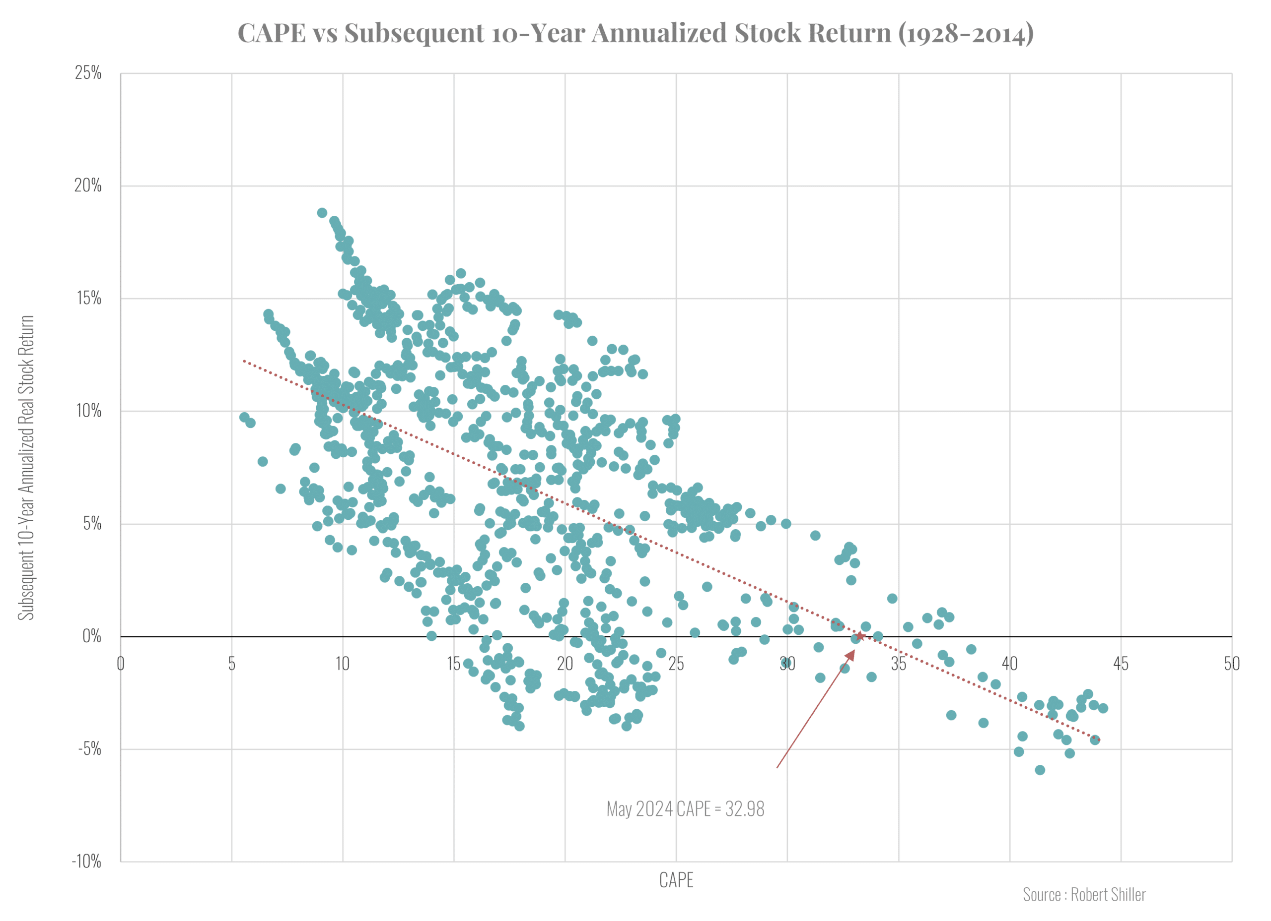
return. It implies that at the current level of the CAPE, 32.98 in May 2024, the total real return for the S&P 500 over the next ten years is basically zero.
Many analysts have used a similar approach employing valuation ratios other than the CAPE. A sophisticated example is the work of John Hussman (2023). Hussman’s key graph is reproduced below as Exhibit 2:
Exhibit 2
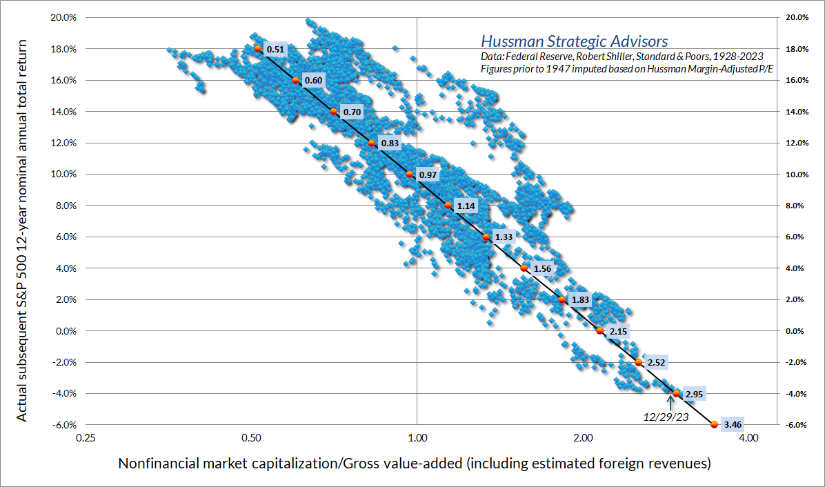
As seen in the graph, at the time of the publication of Hussman’s article, December 2023, the analysis implied an average total return on the S&P 500 over the subsequent 12 years of approximately -4.0% in nominal terms. The prediction was a result of his preferred valuation metric, nonfinancial market capitalization/gross-value added, being close to an all-time high from 1928 to 2024.
As a final example, Research Affiliates has developed an Asset Allocation Model which uses valuation ratios, among other tools, to forecast future long-run stock returns. Like Hussman they predict meager, although not negative, long-run nominal returns for U.S. equity of less than 2 percent over the next decade.
The reason that CAPE analysis, along with the work of Hussman, Research Affiliates, and many others, are predicting such low long-run returns is that current valuations, as assessed by valuation ratios, are exceptionally high. This is clear in both the CAPE and Hussman graphs. In both cases, the current valuation ratio lies on the extreme right-hand side of the exhibit. It is important to recognize that these predictions are not meant to imply that stock returns will be permanently lower. The lower return over the next decade is caused by the fact that the researchers believe that the valuation ratios are “out of whack” and will revert to more normal levels over the next decade. Once the valuation ratios are back to a more normal level, future returns will approximate the long-run historical average.
The predictions based on valuation ratios are fundamentally different from the idea of a structural change. As we shall see, a structural change in key valuation parameters, such as the equity risk premium, can imply that valuation ratios will remain permanently elevated. If that is the case, then forecasts of future underperformance based on valuation ratios reverting toward the mean are misleading. Consequently, it is critical to determine whether the current elevation of valuation ratios is due to a confluence of transitory events, the result of a permanent structural change, or some combination of the two.
The possible structural changes considered here are not the short-term variation in asset prices typically analyzed using Markov models. Instead, the focus is on major long-term changes in the variables that could affect equity valuation over time frames of a decade or more. In that respect, the key challenge is distinguishing a permanent structural change from a slowly mean reverting deviation in the valuation drivers.
To address the question, it is first necessary to determine what might be structurally changing. It is common, for example, to talk about structural change in valuation ratios like the CAPE, but valuation ratios are an output of valuation analysis, not an input. Assuming that markets are relatively rational and efficient, particularly over the long run horizons considered here, the value of a security, or of a market index like the S&P 500, equals the present value of expected future cash flows discounted at an appropriate risk-adjusted rate as shown by equation (1).
P = E(CF1)/(1+k) + E(CF2)/(1+k)2 + E(CF3)/(1+k)3 + … . E(CFn)/(1+k)n + … (1)
For the purposes of this paper, the cash flows and discount rate are stated in real terms. This is based on the assumption that in the long run inflation will be largely neutral. Furthermore, it simplifies the analysis by not having to constantly adjust for changing inflation. Because major structural changes presumably affect most all securities, the analysis here focuses on the overall market as measured by the S&P 500 index.
It follows from equation (1) that there are only three variables to consider as possible candidates for structural change: the growth rate of future cash flows (CF), the real risk-free interest rate and the equity risk premium (together equal k). Structural changes in these variables will then impact valuation ratios such as CAPE.
Starting with the numerator of equation (1), it typically calls for forecasts of cash flow. However, in the long run cash flow and corporate profits are highly correlated, particularly for the aggregate market. There could not be a structural change in one without the other being similarly affected. Because much of the reported macroeconomic data is for corporate profits, that is the variable used here.
Exhibit 3
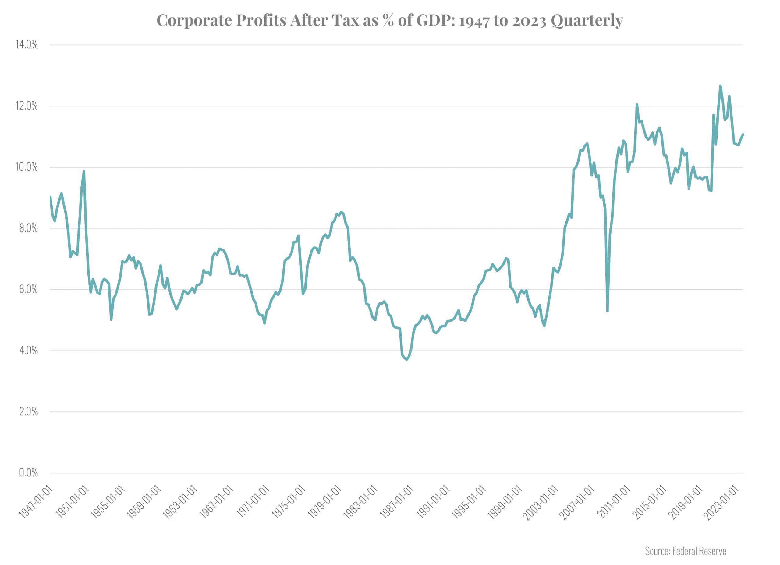
Exhibit 3, which plots corporate after-tax profits as a percentage of GDP, suggests the possibility of a structural change. Whereas the ratio averaged about 6.5% from 1950 through 2003, following the dot.com bust it began to rise. Despite a brief drop during the great financial crisis, the ratio spent most of the years from 2005 through 2023 above 10%. It should be noted that if a structural change in the level of profit occurred, it would cause the level of stock prices to increase, but it would not have an impact on valuation ratios or expected returns. For valuation ratios to be impacted the expected future growth rate of profits must change. In no event would a structural change in future profits affect expected returns on stocks because once information about the change was incorporated into prices there would be no further impact on returns. However, there would be a period of unexpected returns as the market adjusted to the new information about the structural change. With regard to the long-run equilibrium return, equation (1) implies that expected future returns will always equal the discount rate irrespective of the level of or the expected growth of future cash flows.
Exhibit 4
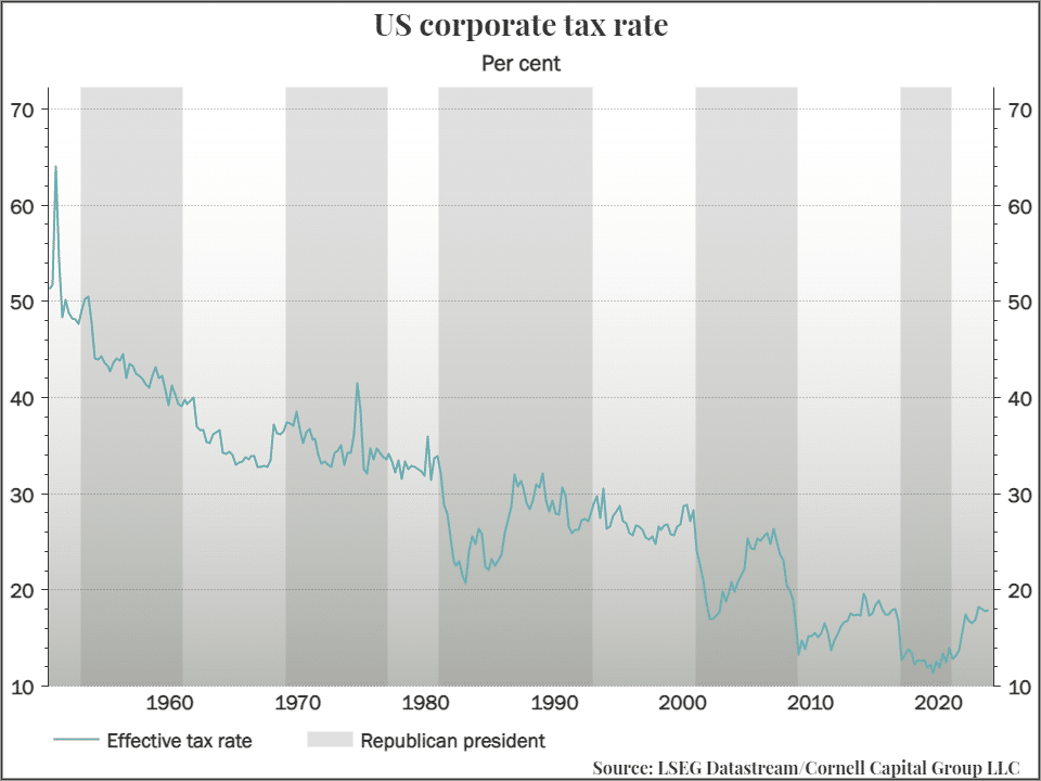
One possible explanation for the increase in corporate profits as a percentage of GDP is a decline in corporate tax rates. Exhibit 4 shows that, in fact, the decline has been dramatic. From a high of over 50% in the 1950s, effective corporate tax rates plummeted to less than 15% under the Trump Administration. Since then, the Biden Administration has increased effective rates somewhat, but they remain below 20%. The key question is whether the existing low rates represent a permanent structural shift or whether rates will revert to the long-run average of about 28%. Currently, the Biden Administration is talking about further increases, but with an election coming up, the outcome is unclear. What is clear is that the United States is running unsustainably large deficits. This suggests that in the long run higher corporate taxes will become a political necessity. If corporate taxes should rise, it will cause a drag on corporate after-tax earnings suggesting a reversion of those earning toward the mean.
Because valuation multiples depend on the future growth rate of earnings not the level, Exhibit 5 examines the growth rate of profits directly. It plots the 10-year rolling compound growth in real corporate earnings from 1957 through 2023. There is no apparent trend in the real growth rate, which averaged about 2.5%. The spikes are due to the financial crisis. A ten-year period that ended with the crisis shows a very low growth rate, whereas a ten-year period that began during the crisis shows a very high growth rate.
Exhibit 5
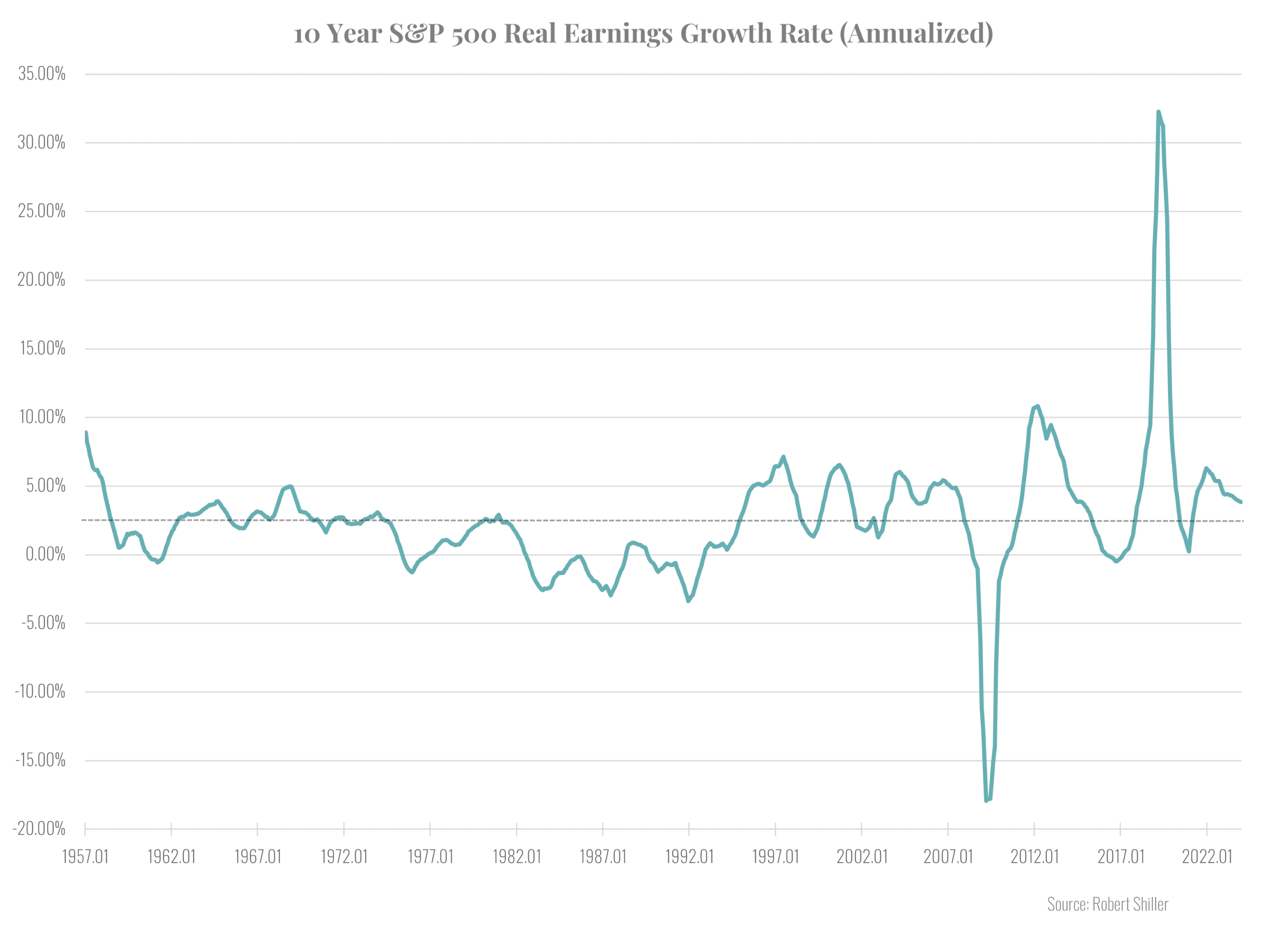
Other than that, the series looks like random variation around the mean value. There is no evidence of a structural change.
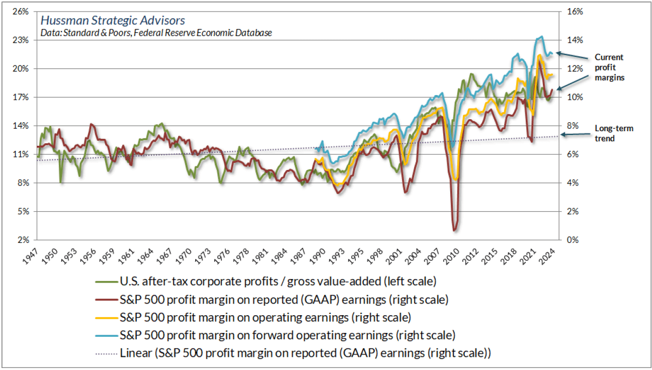
The final measure of profitability is the profit margin. Exhibit 6, taken from Hussman (2024), depicts four measures of the profit margin along with a fitted time trend for the margin calculated from reported GAAP earnings. All the measures tell the same story. Beginning around the turn of the century profits began to rise faster than the long-run trend and, except for a downturn during the financial crisis, continued to do so up to the present. As a result, by 2024 profit margins were at all-time highs. This raises the question of whether the high margins are an anomaly which will mean revert or a permanent change. In addition to the issues of taxes discussed above there are several other reasons for believing that the current level of corporate profit margins is unsustainable.
Exhibit 6
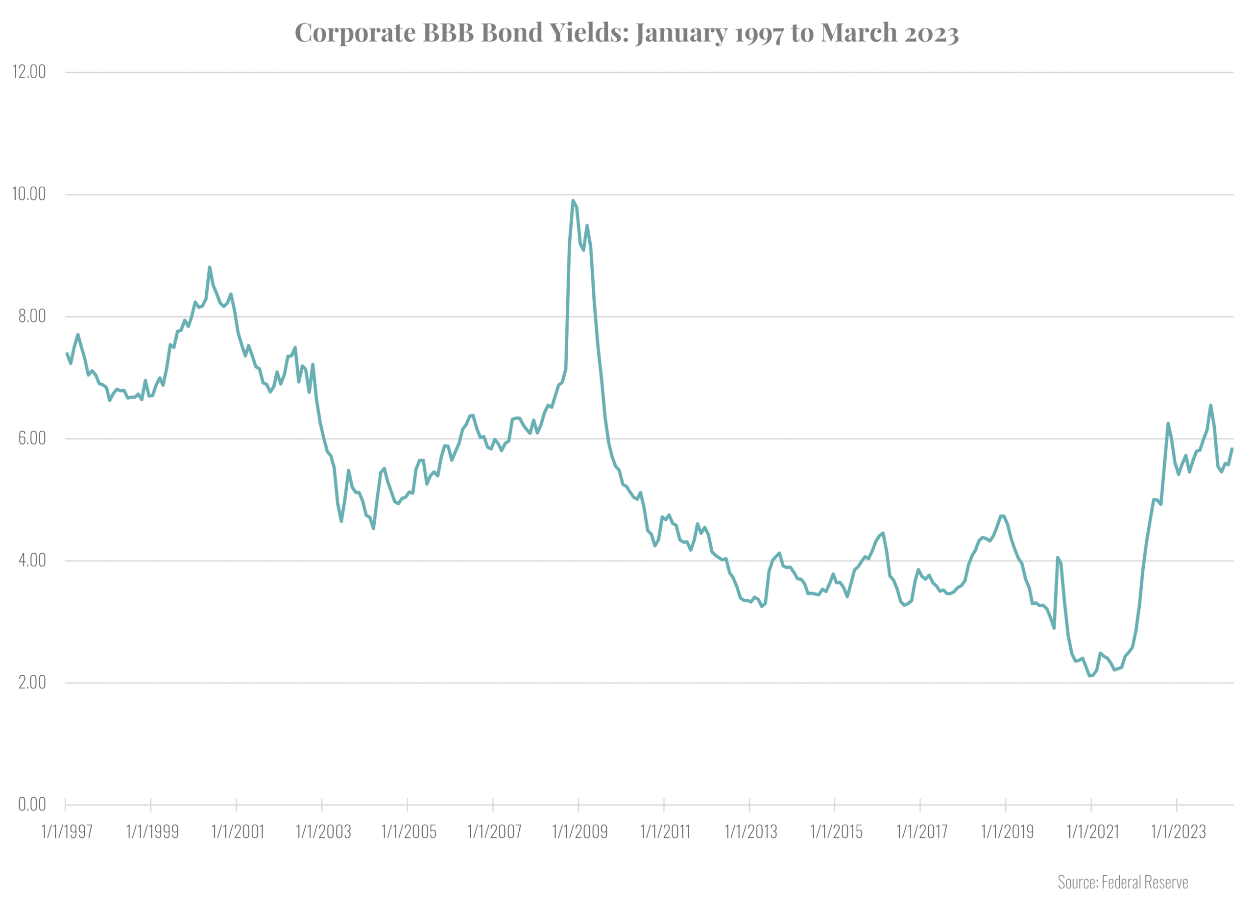
The first is the level of interest rates. Exhibit 7 plots the yields on BBB corporate bonds from January 1977 through March 2024 using data from the Federal Reserve. In recent years, particularly during the pandemic, corporations have been able to reduce interest costs by issuing debt at low yields. However, beginning in 2023 rates turned back up. As existing bonds mature and corporations are forced to refinance at higher rates, profit margins will fall. Based on the previously discussed behavior of interest rates, there is no reason to believe that the companies will be able to borrow at low rates permanently.
Exhibit 7
Second, it is an accounting identity that when one economic sector runs a deficit (that is when spending and investment exceed income) some other economic sector must run a surplus. During the pandemic, households spent well in excess of household income. In part, because the government provided massive subsidies which caused it to run extraordinary deficits. These household and government deficits showed up as a surplus (added profits) for corporations. This is clearly not a sustainable situation. As household and government deficits shrink, corporate profit margins will fall.
In summary, corporate profits measured as a fraction of GDP and corporate profit margins are at record levels. In our view, this is due to a confluence of transitory events and does not represent a permanent structural change in the level of profits. As a result, we believe that regarding corporate profits Hussman and Research Affiliates are on the right track. As profits revert to more normal levels future stock returns are likely to be low during the period of adjustment.
Unlike changes in expected cash flows, structural changes in the discount rate translate one-to-one into changes in expected returns, but the relation is tricky. If the discount rate in equation (1) falls say from 10% to 9%, the immediate impact is an increase in the level of equity prices because the divisor is smaller. This makes it appear as if future returns might be greater because of the large short-term return, but just the reverse is true. Once prices have risen to a new equilibrium level reflecting the smaller divisor, future equilibrium returns will be 9% instead of 10%.
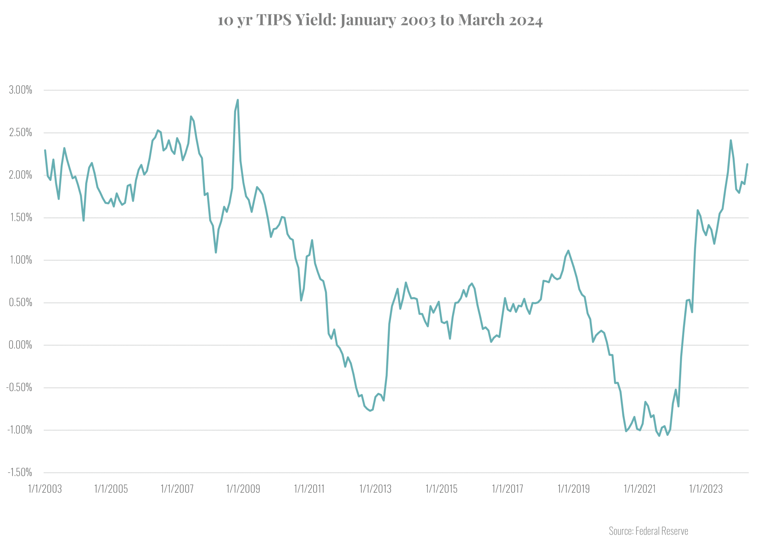
The market discount rate consists of two components, the real interest rate and the equity risk premium. Starting with the real risk-free interest rate, Exhibit 8 plots the real yield on 10-year Treasury TIPS from their inception in January 2003 through March 2024. The TIPS data are the only direct market evidence of the behavior of the real interest in the United States. However, separate data on inflation and interest rates goes back more than a century in the U.S. and back many centuries in the U.K.
The exhibit supports the notion that there were transitory reductions in the real interest rate associated with policy reactions to the great financial crisis and the pandemic, but no permanent change in the level of real rates. This is consistent with many macroeconomic studies which document the ups and downs of real rates but provide little reason to believe that rates will be permanently lower in the future and can, thereby, explain the current high level of stock prices. In fact, the most recent data does not even support the view that current real rates are low by historical standards and thus could not explain the rich equity valuations.
Turning to the equity risk premium, consider an investor contemplating investment in equities in June 1947. They had just experienced a traumatic depression during which stock prices fell 85% followed by a world war. Even in 1947, the S&P 500 stood at 14.84, more than 50 percent below its level of 31.30 prior to the October 1929 crash. Given such circumstances, it would not be surprising if the investor saw equities as an exotic and highly risky investment, one which they would hold only if offered a substantial risk premium.
Exhibit 8
In the ensuing decades, there were many developments which, when considered as a group, would produce a structural change in the long-run equity risk premium. These include, but are not limited to, the following.
- Improvement in capital market regulation and oversight including the establishment of the Securities Exchange Commission. This included new mechanisms for identifying and punishing market manipulation.
- Advances in economic theory and policy leading to a much greater effort by the government to manage the economy, ameliorate recessions, and stabilize financial markets. During the great financial crisis and the pandemic both Congress and the Federal Reserve took theretofore unprecedented steps to combat the economic downturns.
- The accumulation of stock market data demonstrating the performance of equities in the long run.
- Advances in asset pricing and portfolio theory, beginning with the CAPM, leading to improved risk measurement and investment management. This includes breakthroughs in the pricing of derivatives which set the stage for sophisticated hedging strategies.
- The expansion of stock market participation and reduction in the cost of diversification via the invention of mutual funds, exchange traded funds, and the creation of the modern retirement savings system.
- An aging of the U.S. population so that more wealth is held by investors who are willing to accept lower expected returns.
- Significant technological improvements in transacting and record keeping including the invention of electronic trading.
- An increase in stock market liquidity and a decline in the volatility of the return on the market portfolio.
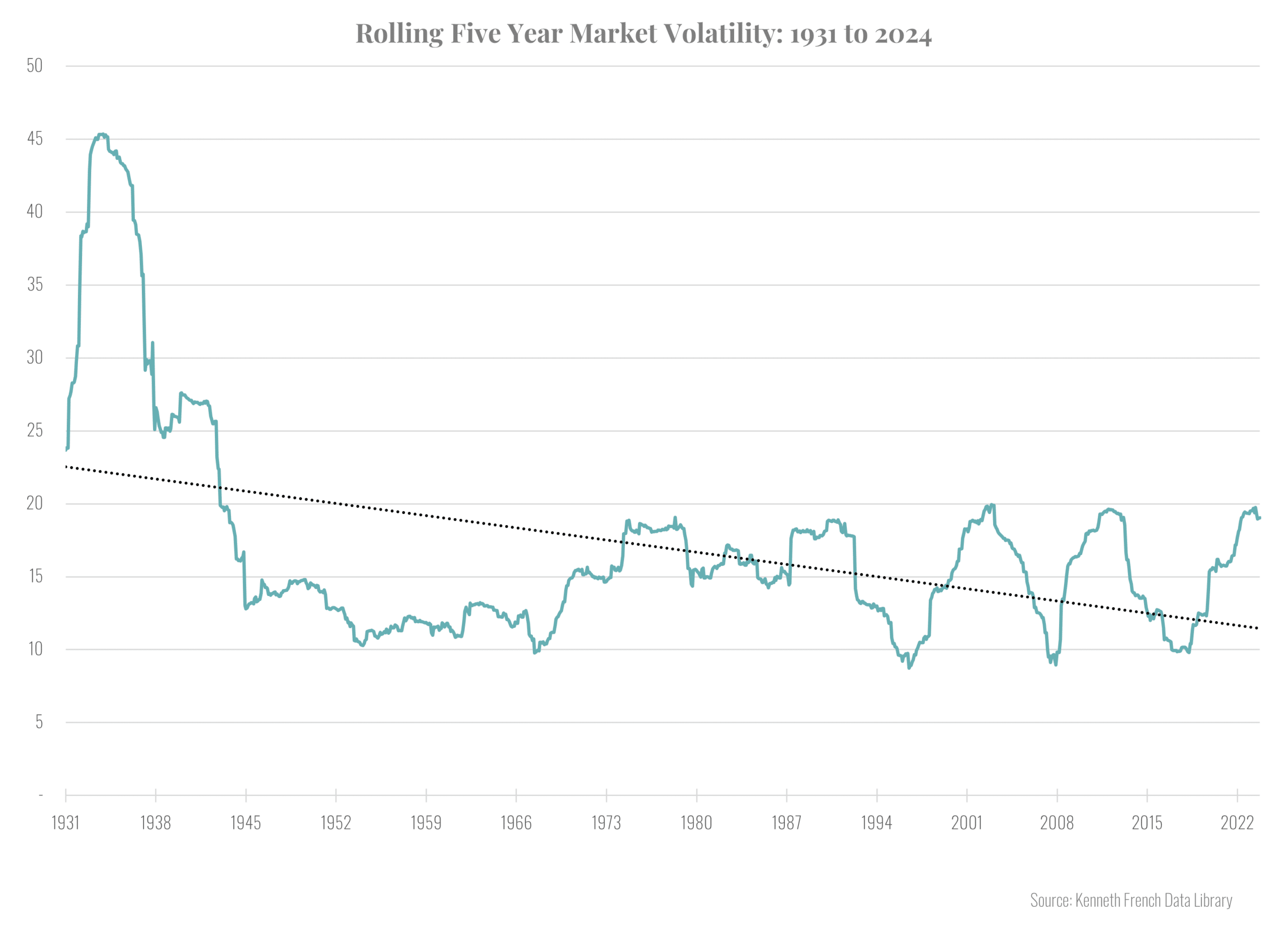
The last point is one for which empirical data is available. Exhibit 9 plots the rolling five-year volatility for the total American stock market using data from Prof. Ken French’s website. It shows that there was a sharp drop in stock market volatility but most of it was prior to 1950. Since then, the volatility has spiked to about 20% during crisis periods and dropped back to 10% during more stable times, without any apparent trend. It should be stressed that ERP would not fall until investors recognized the drop in volatility. It would take a while, perhaps a decade or more, for investors to have sufficient data to conclude that volatility had, in fact, permanently declined.
It is reasonable to conclude that in light of the foregoing observations, that the equity risk premium began a slow decline over the seventy-five years from 1950 through the present. Unfortunately, providing empirical support for this hypothesis is difficult because the ERP is notoriously difficult to estimate. First, if it changes over time, as we argue it has, then historical estimates mix apples and oranges because different time periods have different ERPs. One way to combat this is to use short historical time periods to estimate the ERP so as to limit the impact of the changes. Unfortunately, estimates of the ERP using estimation periods even as long as a decade are so noisy that meaningful statistical conclusions cannot be drawn. A better approach is to estimate the implied equity risk premium as described by Prof. Aswath Damodaran (2024).
Exhibit 9
This approach solves for the level of the discount rate that equates the present value of future earnings estimates with the current market price. Though an improvement, this approach is not a panacea. It requires a projection of future earnings and an estimate of what fraction of those earnings are paid out to investors. Estimating the payout ratio, in turn, requires taking account of the rise of buybacks as a method for distributing cash.
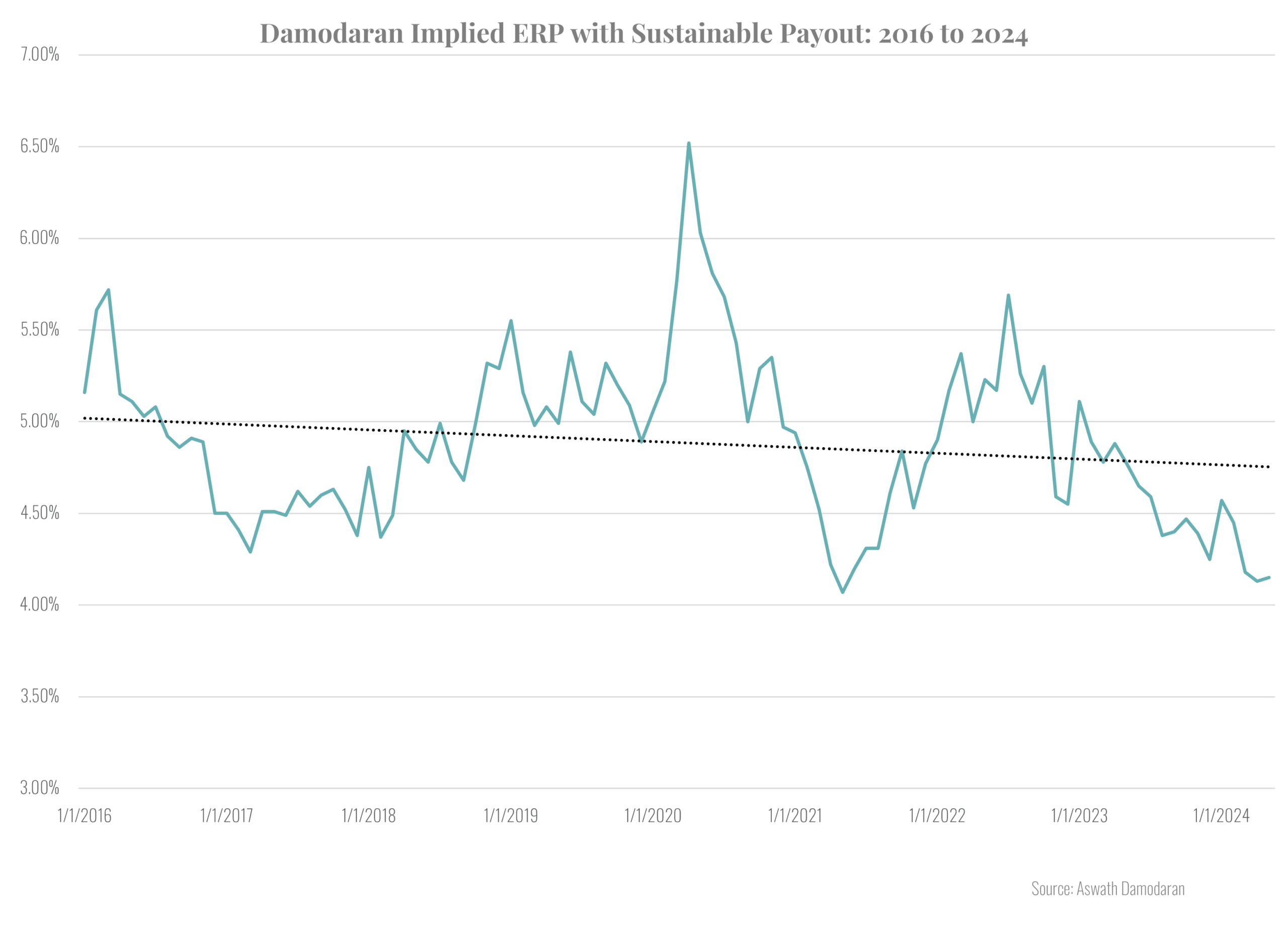
As an example of this approach, Exhibit 10 plots Damodaran’s estimate of the ERP using what he terms sustainable payout ratios. Unfortunately, this estimate is available only back to January 2016. Although the estimated ERP does show some evidence of decline, it is hard to draw a meaningful conclusion due to the short time period and the high volatility of the data.
Exhibit 10
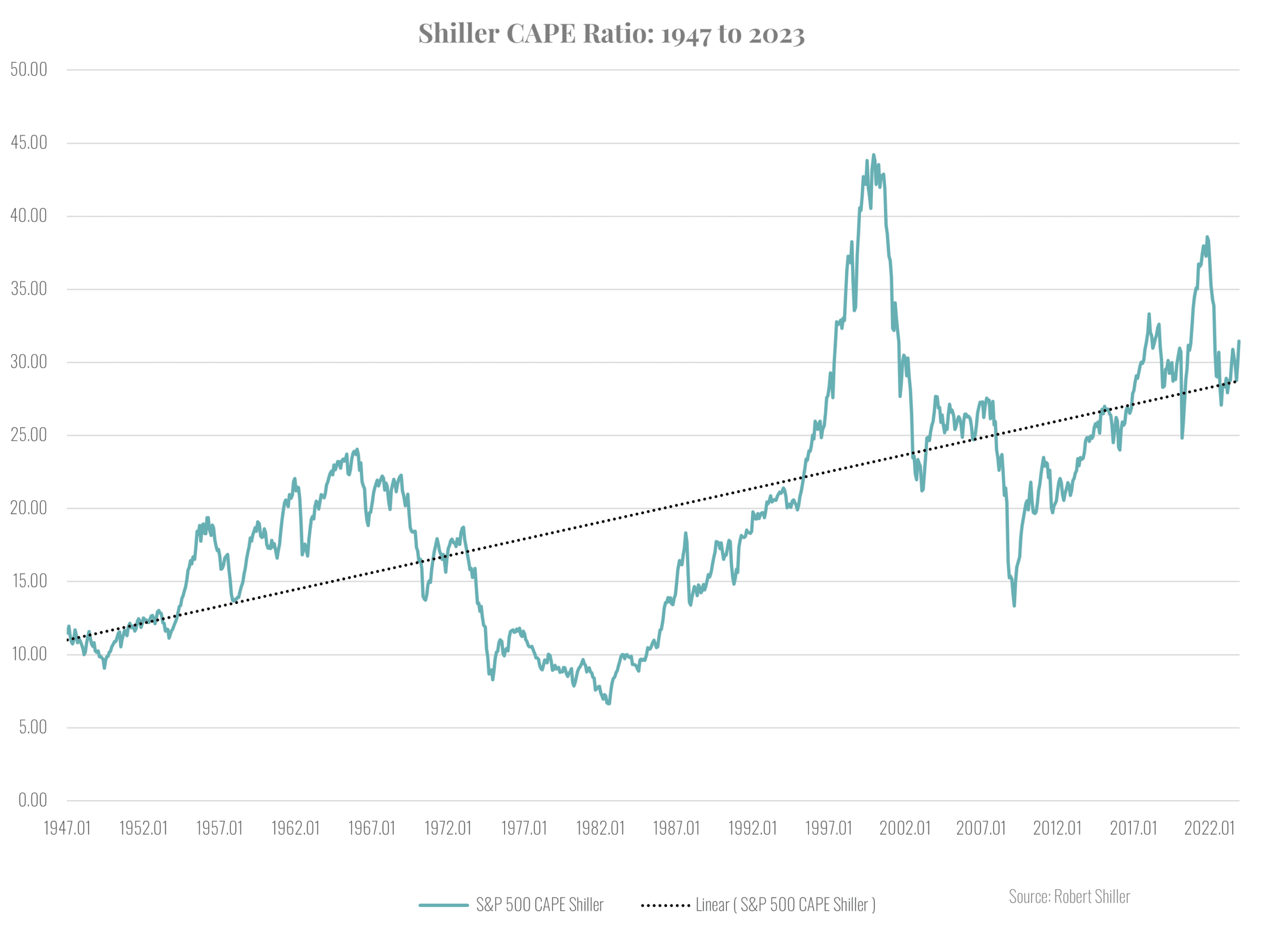
An alternative is not to try to estimate the ERP directly, but to look for its impact on valuation ratios. A slowly declining ERP, amid a lot of noise, will lead to a related rise in valuation ratios along with the associated noise. For instance, Exhibit 11 plots the Shiller CAPE ratio from 1947 through 2023. To be sure, there is a lot of short-term variation in the CAPE, but there is also evidence of a slow, persistent upward trend consistent with a slow, persistent decrease in the ERP. In our view, this evidence along with the theoretical points made earlier, support the conclusion that there has been a structural change in the level of the equity risk premium.
Exhibit 11
It is important to appreciate the impact that a relatively small change in the ERP can have on equity valuation, especially starting at low levels. For example, applying a valuation model that we have developed at the Cornell Capital Group reveals that a one percentage point drop in the ERP, from current levels, leads to an almost 20% increase in the level of stock prices and associated valuation ratios.
Recognizing the importance of a structural change in the ERP has important implications for investors. As Antti Ilmanen (2022) notes, the persistently richening market valuation between 1950 and 2020 made contrarian investors meaningfully underinvested in the equity premium. Those investors expected valuation normalization and so limited their market exposure, but the normalization never came. That is because the richening was apparently due to a permanent decrease in the ERP, not transitory factors.
In stressing the importance of a long-run decline in the ERP, the short-run variation should not be overlooked. Turning back to the plot of Damodaran’s implied ERP, there is a great deal of short-run variation around the slowly declining trend line. Furthermore, the current level is below the trend line. This means that regression toward the mean is also likely to occur in the case of the ERP, but the regression will be toward a lower mean.
Summary and Investment Implications
Based on the high current level of stock prices as assessed by the valuation ratios, many market analysts including Hussman Strategic Advisors and Research Affiliates are projecting low or even negative returns on the S&P 500 over the next decade. These projections are based on the historical observation that when valuation ratios are high, long-run future returns are low. That conclusion rests, in part, on the assumption that current conditions do not reflect a structural change. If a structural change has occurred, then historical relations could be a misleading indicator of future returns. In particular, if there is a fundamental reason for prices to be permanently higher, then future returns will not be lower despite the current high valuations.
Talking about structural change is pointless without specifying what is allegedly changing. The fundamental discounted cash flow valuation equation makes it clear that for a structural change to impact equity pricing it must affect either the growth in expected future cash flows, the real interest rate, or the equity risk premium. The question is whether a permanent structural change in any of these variables can explain the current elevated level of stock prices. If it can, then there is no reason for long-run future returns to be low. Taking the variables one-by-one, we see no evidence to support the argument for a structural change in the real interest rate. The situation regarding corporate profits is more nuanced. Both corporate profit margins and corporate profits as a fraction of GDP are near historical highs. The question is whether that represents a permanent change in the underlying economics or a confluence of transitory events. There is no unambiguous answer to the question, but we favor the transitory explanation. If that is true, then a reversion of profits toward the mean should lead to lower long-run stock returns as predicted by Hussman and Research Affiliates during the period of transition. The final variable is the equity risk premium. Here we argue that the ERP has undergone a slow decline over the period since 1950. However, that decline is mixed with significant short-term variation. We believe that the current level of the ERP reflects a combination of a long-run decline with a short-term drop.
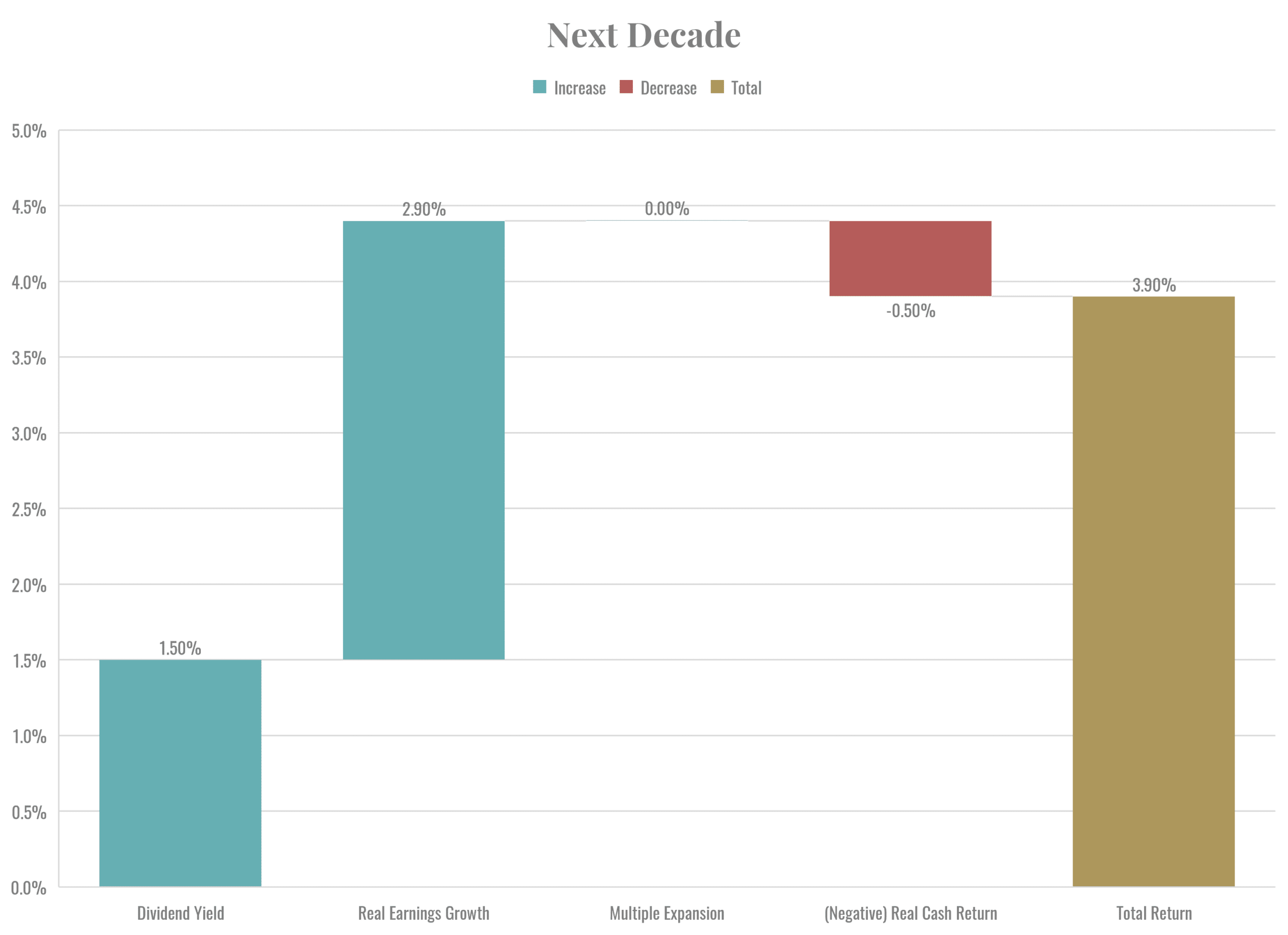
The bottom-line question is how to put all the pieces we have analyzed together. One way to do that is based on the approach we described in our Reflections on Investing. As shown in Exhibit 12, the future return on the S&P 500 in excess of the return on cash over the next decade can be broken down into four parts: the dividend yield, real earnings growth, multiple expansion, and the real return on cash. If the entire increase in valuation multiples were due to a permanent structural change, then it is reasonable to assume that in the upcoming decade the multiples would remain at their current elevated level, so that future expansion would be zero as shown in the exhibit. We also assume that the dividend yield will remain at its current level of 1.5% and that real earnings growth will equal its long-run historical average of 2.9%. With respect to the real return on cash, the Federal Reserve projects it to be negative 0.5% because the nominal cash yield is forecast to be less than the rate of inflation.
Putting all the pieces together, the projected future stock return in excess of the cash yield comes to 3.9%. Because the nominal yield on cash is projected to be about 2%, the total predicted nominal return comes to 5.9%. That number is meager, but it is substantially greater than the number produced by the CAPE analysis or by Hussman and Research Affiliates. However, the calculation was performed assuming that a permanent structural change accounted for all the increase in the valuation multiple.
Exhibit 12
In fact, the data presented here support the hypothesis that much of the increase in the multiple was due to transitory factors. It is reasonable, therefore, to expect reversion toward the mean during the upcoming decade. As an example, the mean of CAPE during the period from 1947 through May 2024 is 19.93 and the mean from the bubblier period from 1990 to the present is 26.62. For the valuation multiple to revert to the long-run mean over the next ten years it would have to fall an average of 4.9% per year. Reverting to the shorter-run mean would require a drop of 2.1% per year. These declines reduce the expected return over the next ten years to a range of 1.0% to 3.8% per year. Because we believe there was a structural decline in the ERP, that was accompanied by transitory drop, the 3.8% would be our best estimate of the S&P 500 total nominal return over the next decade. This is well below the nominal compound return from the previous decade of 12.76%. It is also less than the current ten-year Treasury rate of 4.5% indicating a negative risk premium during the upcoming decade.
Our long-run analysis should not be interpreted as a short-run projection. For example, there are a lot of ways that the average return on the market could be 3.8% over the next ten years. One path would be to experience annual returns on the order of 3.8% throughout the decade. Another quite different path would be to have a short-term crash followed by more normal market returns on the order of 9% per year. Our long-run analysis does not allow us to predict which of those two paths, or any other path that produces an average return of 3.8%, is more likely.